8. Hillslope hydrology and BGC impacts breakout group

8.1. Objectives of the workshop breakout

Objectives of this workshop breakout is learn how to set up and run ELM simulations to explore a set of four ELM configurations:

ID	Features	Spatial Extent	Spatial Resolutions	Configuration name (CODE)
IM0_DS0	Topounits	Panarctic	0.5 deg	Baseline (IM0_DS0)
IM0_DS1	Topounits + meteorology downscaling	Panarctic	0.5 deg	Met. Downscaling (IM0_DS1)
IM1_DS0	Topounits + IM2 hillslope hydrology	Panarctic	0.5 deg	Hillslope Hydrology (IM1_DS0)
IM1_DS1	Topounits + meteorology downscaling + IM2 hillslope hydrology	Panarctic	0.5 deg	Met. Downscaling + Hillslope Hydrology (IM1_DS1)

8.2. Background on ELM features we will explore

8.2.1. Topounits

Topography-based subgrid scheme (or Topounits) and methods for downscaling of atmospheric forcings were introduced in ELM by Tesfa et. al. 2024 to better resolve terrestrial processes in regions of heterogeneous terrain.

Tesfa, T. K., Leung, L. R., Thornton, P. E., Brunke, M. A., & Duan, Z. (2024). Impacts of Topography‐Based Subgrid Scheme and Downscaling of Atmospheric Forcing on Modeling Land Surface Processes in the Conterminous US. Journal of Advances in Modeling Earth Systems, 16(8). https://doi.org/10.1029/2023ms004064

Tesfa et. al. 2024 derived topounits from high resolution elevation data (90 m) for the half degree grids. Topounits‐based surface properties (including PFTs, soil texture etc.) input parameters were generated by mapping grid‐level values onto the TGUs of each grid.

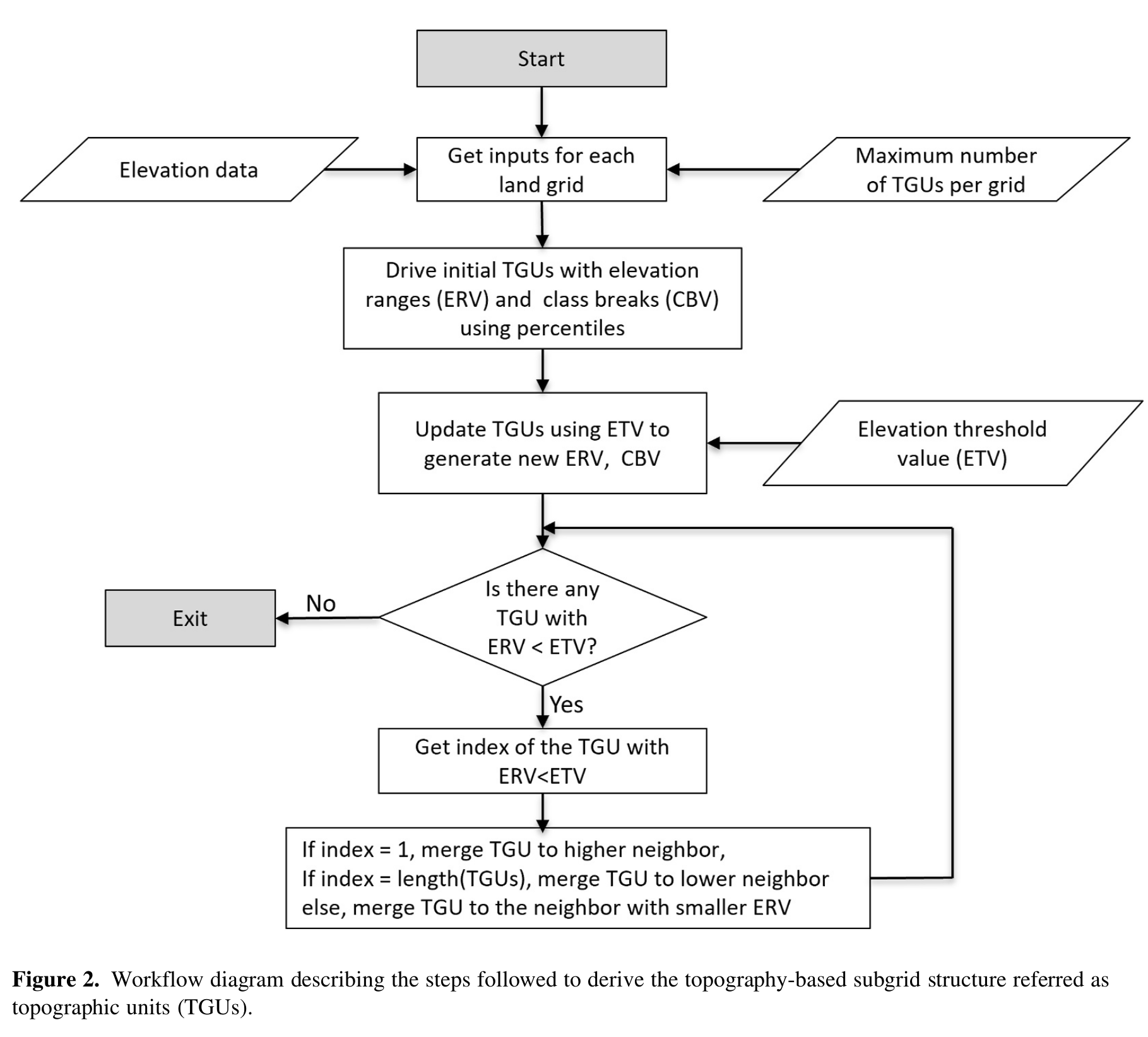
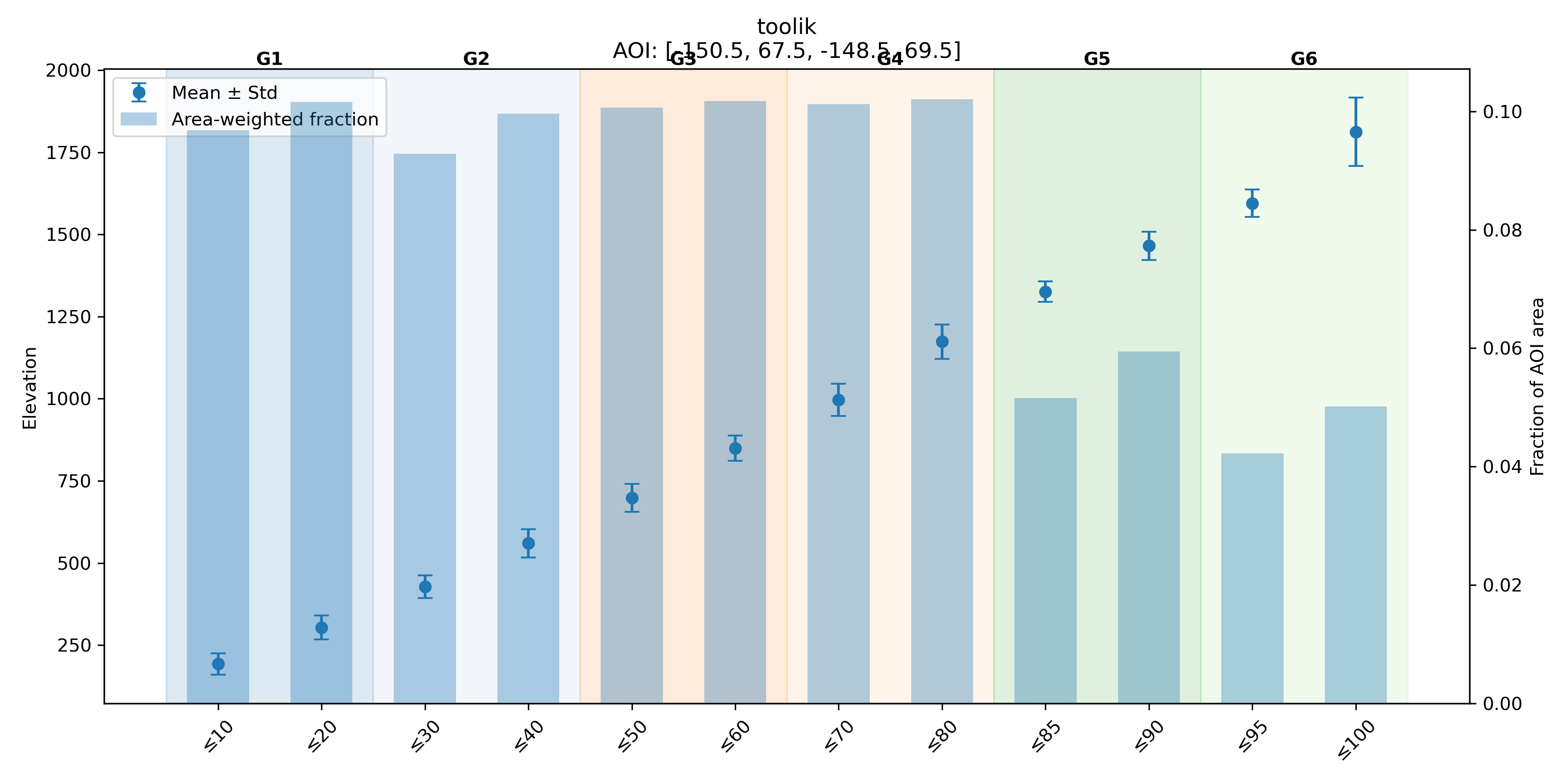
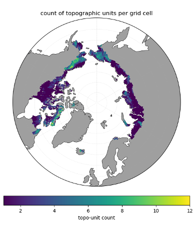
The algorithm extracts elevation values based on the boundary of the modeling unit (grid) and discretizes the modeling unit into 12 initial subgrid units using the 12 percentile elevation values calculated to represent the elevation values at each consecutive percentile (10th, 20th, 30th, 40th, 50th, 60th, 70th, 80th, 85th, 90th, 95th and 100th). Then, the 12 values of elevation range are determined using the minimum elevation value within each grid and the corresponding percentile elevation values as class breaks. Furthermore, the 100‐m elevation threshold value is used to calculate new values of elevation class break using a recursive algorithm developed by Tesfa et. al. 2024. The recursive algorithm merges any elevation class with elevation range less than the threshold value to its neighboring class recursively until all the classes with elevation range smaller than the threshold value are removed. This allows the topography‐based subgrid scheme to capture the impacts of topographic heterogeneity while minimizing computational demand of the model by varying the number of topounits per grid depending on the topographic heterogeneity within each modeling unit.

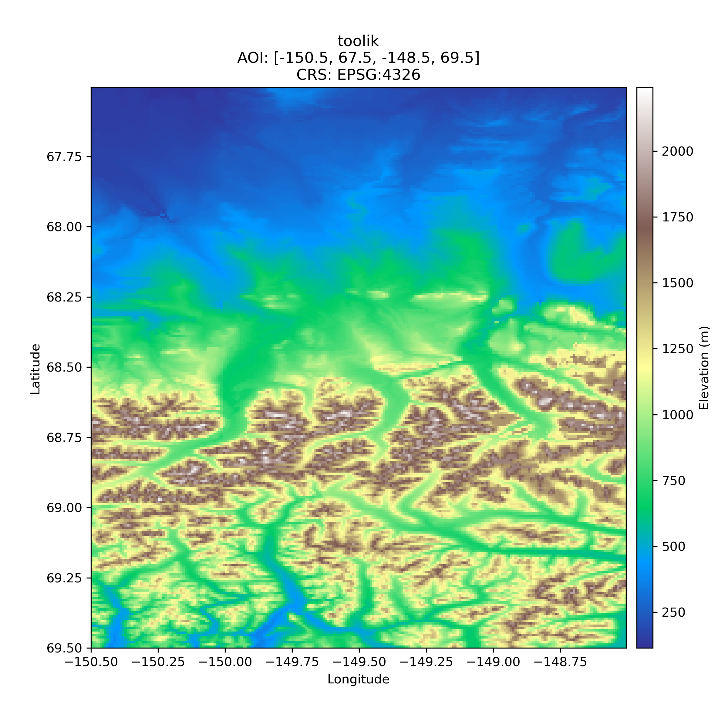
Digital Elevation Model (DEM) near Toolik Field Station

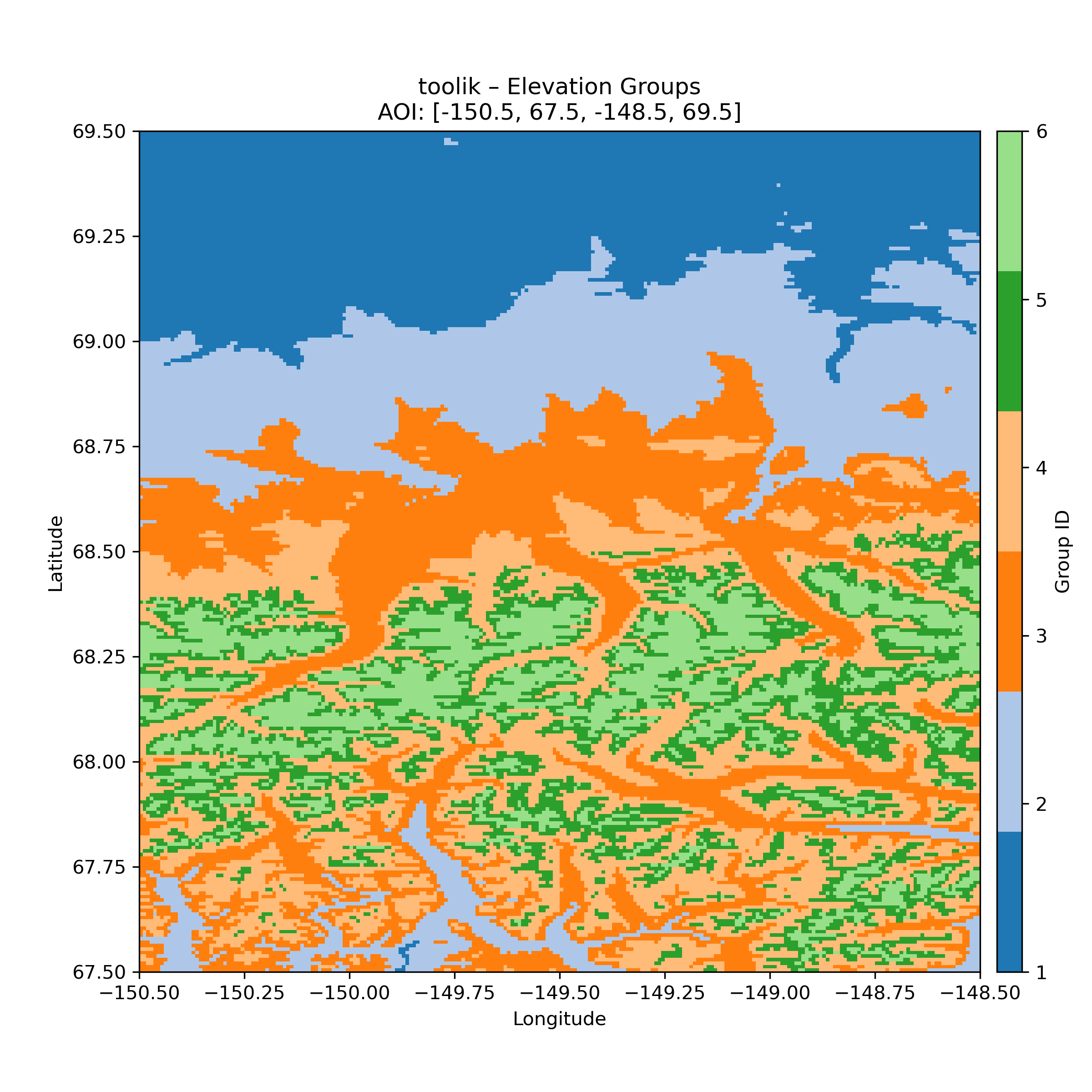
Topounits (recursive merging) for Toolik Field Station identify 6 topounits

Plot below show the 12 percentile based elevation bins and the recursive merge strategy to create the topounits.

Plot below shows the number of topounits across a 0.5 degree Pan-Arctic ELM grid.

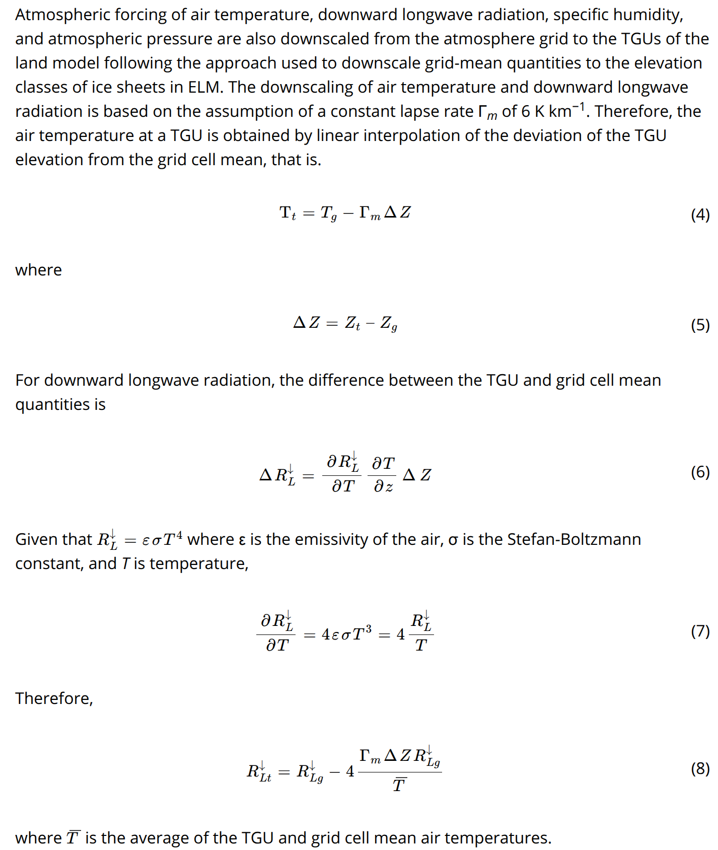
8.2.2. Atmospheric Downscaling Scheme

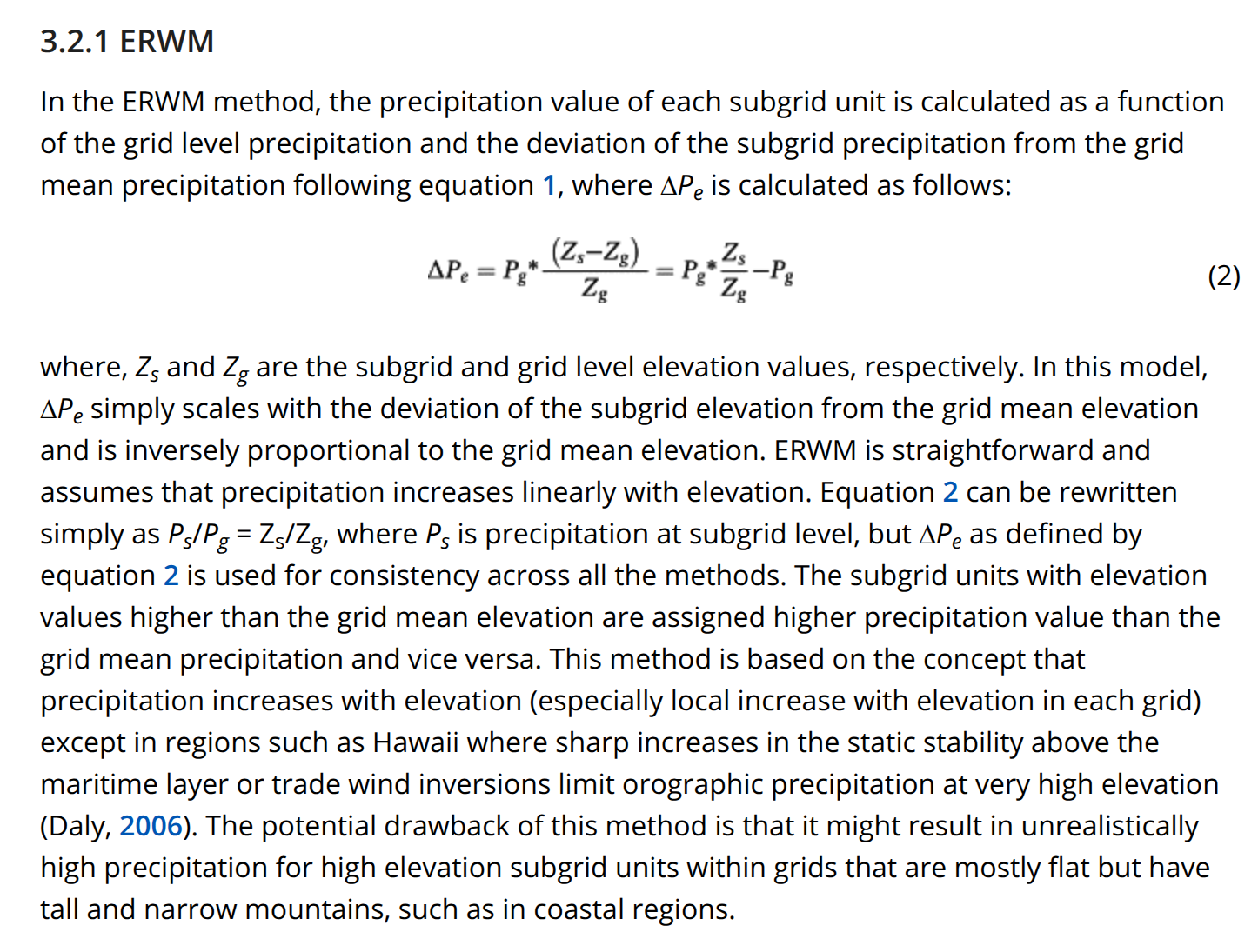
Elevation Range with Maximum elevation Method (ERMM) devveloped by Tesfa et. al. 2020 is used to downscale atmospheric forcings from gridcell to topounits. The ERMM method uses only the topographic characteristics of the grid and the TGUs to disaggregate grid-level precipitation to the TGUs of the grid.

Tesfa, T. K., Leung, L. R., & Ghan, S. J. (2020). Exploring topography-based methods for downscaling subgrid precipitation for use in Earth System Models. Journal of Geophysical Research: Atmospheres, 125, e2019JD031456. https://doi.org/10.1029/2019JD031456

8.2.3. IM2 Hillslope Hydrology

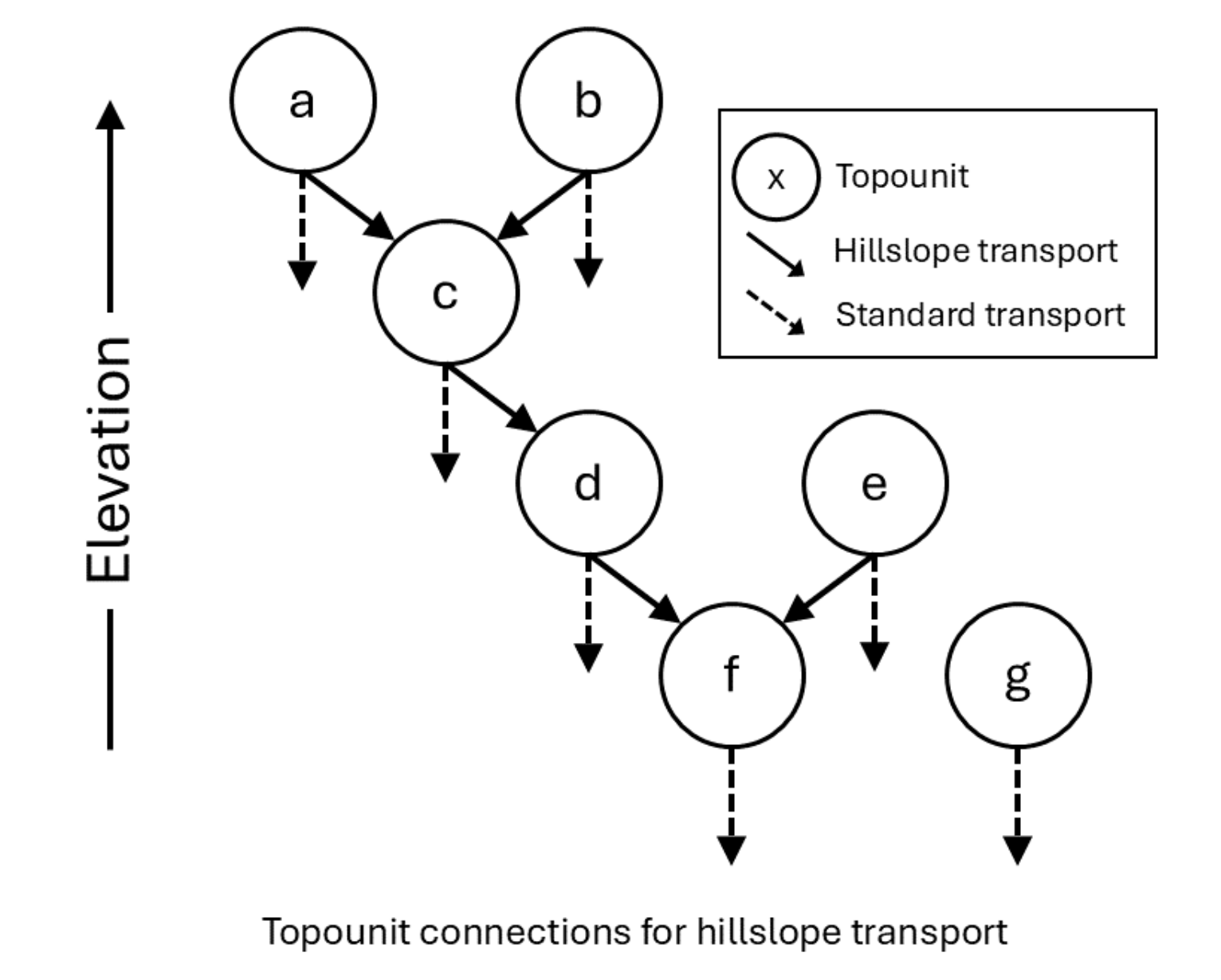
Connections among multiple topounits (labeled a through g) on a single gridcell. Each topounit is connected to at most one other downhill topounit (the next lowest in elevation), while the lowest topounit does not have a downhill connection.

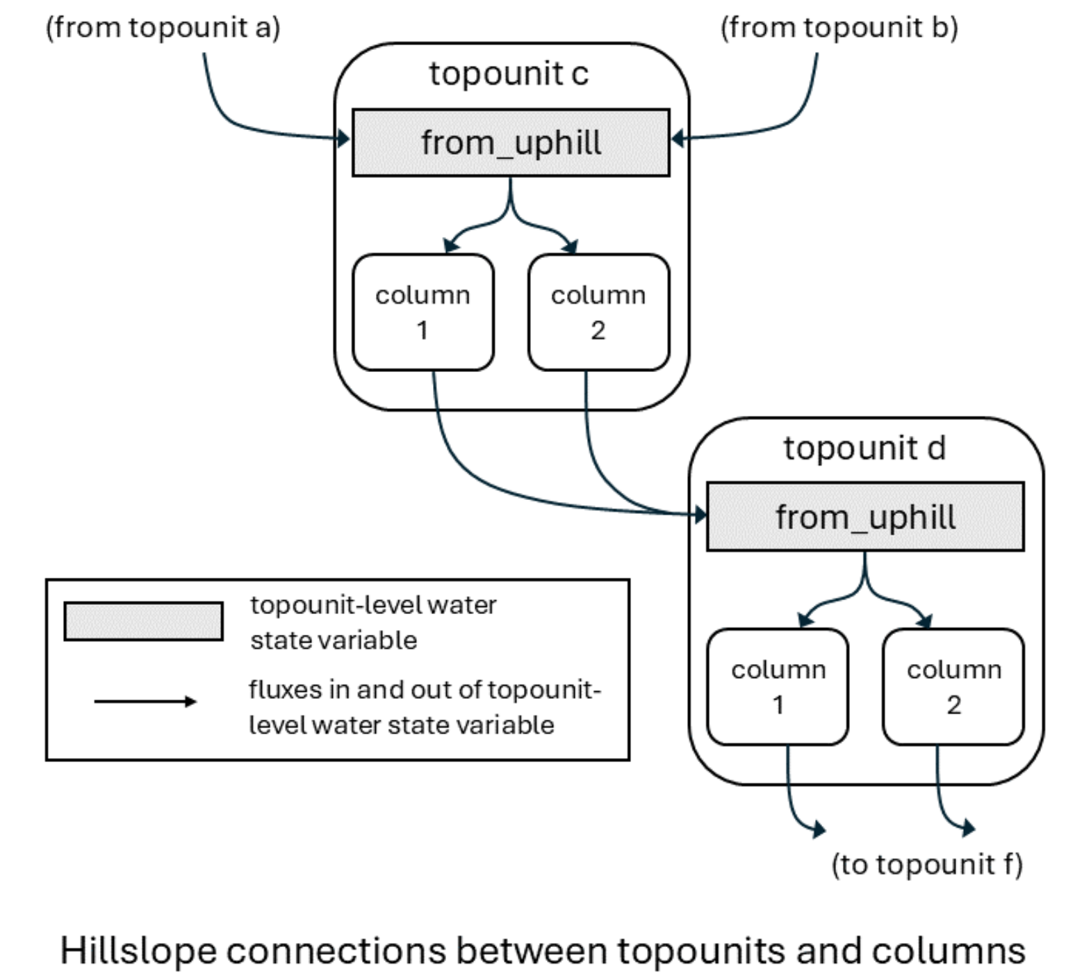
Arrangement of topounits, columns, state variables, and water fluxes

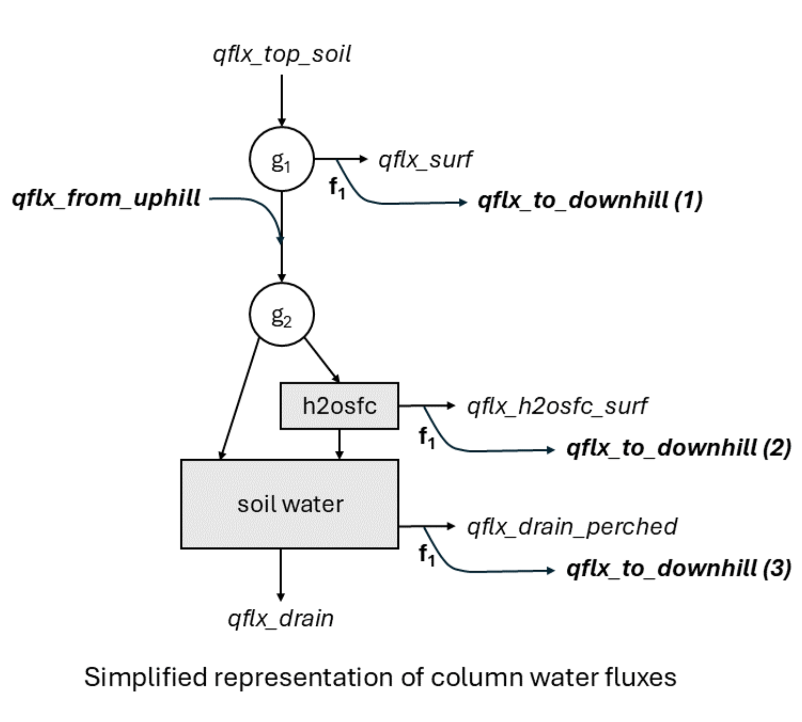
A summary of water fluxes for a single column.

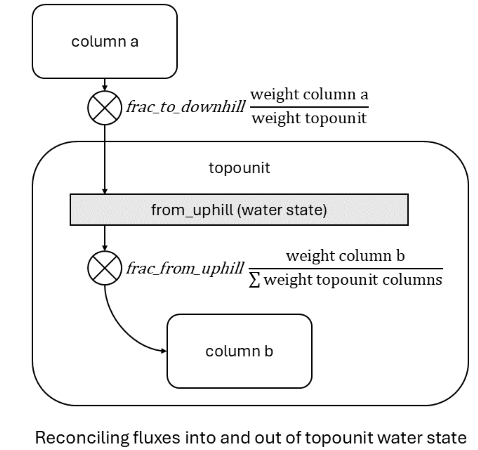
Summary representation of hillslope hydrology fluxes at the topounit level. The water state variable for one topounit (gray shaded box) receives water from a column on an uphill topounit (column a). The operator symbol represents combined user parameter for the fraction of column-level flux to transport downhill and the scaling factor accounting for potential difference in area between the upstream column and the downstream topounit. Water leaving the topounit water state is moved to columns on the topounit .

8.3. Running ELM

We will use Council C71 site (at Seward Peninsula of Alaska) for all simulations in this exercise. To run ELM in offline mode (without coupling to other E3SM components), we would need input datafiles as summarized below:

https://github.com/ORNL-Ecosystem-Projects/Documentations/wiki/Offline-ELM-Inputs-for-Regional-Simulations

Described below are the essential data components need for this exercise.

8.3.1. ELM Domain Files

ELM domain file is located within the container volume at: /mnt/inputdata/E3SM/share/domains/domain.clm/

Files used in this exercise include the identifier ‘C71’ for Council Mile Marker 71, at Seward Peninsula of AK, AK in their name:

domain.lnd.r05_RRSwISC6to18E3r5.240328_C71-Grid.nc: This file provides the computational mesh for ELM, including grid location and its size (vertices, and area).

8.3.2. ELM Surface Datasets

ELM requires a number of land surface properties to be defined in netCDF files that are located at: /mnt/inputdata/E3SM/lnd/clm2/surfdata_map

topounit_surfdata_0.5x0.5_simyr1850_c20220204_C71-GRID.nc: Contains the datasets with “topounits” to be used in this exercise.

8.3.3. ELM Forcing Files

A number of meteorological datasets are being used by NGEE-Arctic to provide forcings for the ELM simulations. This exercise will use GSWP3 (v2) data, available at: /mnt/inputdata/E3SM/atm/datm7/gswp3/

Data for Council site are within the subdirectory: cnl/

There are 7 key meterological variables at 3 hourly frequency that provides meteorological:

FSDS	incoming solar shortwave radiation
FLDS	incoming solar longwave radiation
PRECTmms	precipitation in unit of mm/s
PSRF	air pressure (near-surface)
QBOT	air specific humidity (near-surface, or bottom of atmosphere)
TBOT	air temperature
WIND	wind speed

8.4. Running ELM: Exercises on topographic unit, hereafter, topounit, data and functionality

A general briefing on how to use or run ELM may be found in: https://github.com/ORNL-Ecosystem-Projects/Documentations/wiki#welcome-to-the-e3sm-land-model-elm-pflotran-coupled-wiki

In this exercise we will conduct ELM runs at a single NGEE Arctic Phase 4 evaluation site: Council, Council Road Mileage 71, AK.

site name	council
site code	AK-SP-CL71
meteorological forcing source	GSWP3

domain file	/mnt/inputdata/E3SM/share/domains/domain.clm/domain.lnd.r05_RRSwISC6to18E3r5.240328_C71-Grid.nc
surfdata file	/mnt/inputdata/E3SM/lnd/clm2/surfdata_map/topounit_surfdata_0.5x0.5_simyr1850_c20220204_C71-GRID.nc
inidata file	/mnt/inputdata/E3SM/lnd/clm2/inidata/council/topounit_gswp3_AK-SP-CL71_ICB1850CNPRDCTCBC.elm.r.0601-01-01-00000.nc

We will work through the following steps:

1. A full-run of 3 stages (AD spinup, final spinup, transient run) of ELM simulation, but for only a few years (due to time constraint).

2. Create a transient case, build it, but not run.

3. Perform 4 sets of simulations, using the case setup and built in #2.

8.4.1. A sample end-to-end topounit enabled ELM run

docker run -it --rm \
  -v $(pwd):/home/modex_user \
  -v inputdata:/mnt/inputdata \
  -v output:/mnt/output \
  yuanfornl/ngee-arctic-modex26:models-main-latest \
  /home/modex_user/model_examples/ELM/run_ngeearctic_site.sh \
  --site_name=council \
  --topounits_atmdownscale \
  --case_prefix=topounit \
  --met_source=gswp3 \
  --ad_spinup_yrs=20 \
  --final_spinup_yrs=10 \
  --transient_yrs=10

--topounits_atmdownscale, will turn ON the feature to downscaling air temperature and precipitation from gricells to topounits.

--ad_spinup_yrs=20, --final_spinup_yrs=10, --transient_yrs=10 defines the number of years simulation should be conducted for ad_spinup, final_spinup, and transient steps. These values typically would be higher, but set low for illustration.

Topounits and downscaling features can have significant impact on hydrological processes, and consequent impacts on biogeochemical cycle, if multiple topounits are properly created in ELM surface data. We will look into those effect later in this exercise.

8.4.2. Create a new transient case and build it.

docker run -it --rm \
  -v $(pwd):/home/modex_user \
  -v inputdata:/mnt/inputdata \
  -v output:/mnt/output \
  yuanfornl/ngee-arctic-modex26:models-main-latest \
  /home/modex_user/model_examples/ELM/run_ngeearctic_site.sh \
  --site_name=council \
  --topounits_atmdownscale \
  --case_prefix=topounit \
  --met_source=gswp3 \
  --ad_spinup_yrs=0 \
  --final_spinup_yrs=0 \
  --no_submit

The option,

--ad_spinup_yrs=0 will allow workflow to SKIP the step of biogeochemically accelerated spinup.

--final_spinup_yrs=0 will SKIP stage of normal spinup.

It will create a case for transient simulation. --no_submit will however tell the workflow not start the simulation, which we will do in the next step..

The above command will generate 3 directories for the case: CASE = topounit_gswp3_AK-SP-CL71_ICB20TRCNPRDCTCBC

CASEROOT: /mnt/output/cime_case_dirs/topounit_gswp3_AK-SP-CL71_ICB20TRCNPRDCTCBC EXEROOT: /mnt/output/cime_run_dirs/topounit_gswp3_AK-SP-CL71_ICB20TRCNPRDCTCBC/bld RUNDIR: /mnt/output/cime_run_dirs/topounit_gswp3_AK-SP-CL71_ICB20TRCNPRDCTCBC/run

EXEROOT is the root directory where the cose is built and the main executable e3sm.exe is located.

RUNDIR contains the outputs of the simulation. We will access the outputs from this directory during analysis and visualization step.

8.4.3. Conduct ELM Simulations

Four simulations we would conduct explore three key features of ELM, in various combinations:

1. Use of topounits to capture subgrid scale topographic variability

2. Atmospheric downscaling for elevation based downscaling of grid cell level forcings to topounits.

3. NGEE-Arctic developed IM2 module for hillslope hydrology.

We will use the Field-to-Model: model_examples/ELM/run_ngeearctic_site_rerun.sh with various flags to conduct all these simulations.

RUN 1: Baseline (IM0_DS0)

docker run -it --rm \
  -v $(pwd):/home/modex_user \
  -v inputdata:/mnt/inputdata \
  -v output:/mnt/output \
  yuanfornl/ngee-arctic-modex26:models-main-latest \
  /home/modex_user/model_examples/ELM/run_ngeearctic_site_rerun.sh \
  --case_name=topounit_gswp3_AK-SP-CL71_ICB20TRCNPRDCTCBC \
  --case_dirs=/mnt/output/cime_case_dirs \
  --run_type=branch \
  --restart_path=/mnt/inputdata/E3SM/lnd/clm2/inidata/council \
  --restart_case=topounit_gswp3_AK-SP-CL71_ICB20TRCNPRDCTCBC \
  --restart_date=2005-01-01 \
  --continue_run_yrs=10 \
  --rest_yrs=11 \
  --user_namelist="topounit" \
  --merged_ncfile="MasterE3SM_subgrid.out_met-ds-NO_IM-2-NO_yes.topounit_gswp3_AK-SP-CL72_ICB20TRCNPRDCTCBC_2005.2014.nc"

--case_dirs, --case_name: will be set to the CASEROOT, we created in previous steps.

--run_type=branch: This must be used together with --restart_path, --restart_case, --restart_date

branch RUN_TYPE is one of 3 types supported by the workflow (startup, restart, and branch). It will find data and rpointer files at --restart_path, with case_name == --restart_case, and start a simulation from the date specified by --restart_date.

--continue_run_yrs=10: Would perform a simulation for 10 years. So if starting from 2005-01-01, it will end on 2014-12-31.

--rest_yrs=11: Tells the model to save restart files every 11 years. Since the current run only goes for 10 years, it won’t generate any restart files. .. If intended to, have to set this to not greater than –continue_run_yrs.

--user_namelist="topounit": Enables topounits feature .. , but no meteorological downscaling or IM2 hillslope hydrology

--merged_ncfile will asks workflow to save merged sub-grid output netCDF files to this file. Otherwise, default filename would be ELM_output_PFT.nc (overwriting any existing file with that name).

It can be any name. Here we will use names with some identifiable tags, e.g. E3SM version, not-grid-aggregated, met-ds (NO), IM-2 (NO), topounit (yes), met. type, site-code, ELM compset, period, etc.

RUN 2: Downscaling (IM0_DS1)

docker run -it --rm \
  -v $(pwd):/home/modex_user \
  -v inputdata:/mnt/inputdata \
  -v output:/mnt/output \
  yuanfornl/ngee-arctic-modex26:models-main-latest \
  /home/modex_user/model_examples/ELM/run_ngeearctic_site_rerun.sh \
  --case_name=topounit_gswp3_AK-SP-CL71_ICB20TRCNPRDCTCBC \
  --case_dirs=/mnt/output/cime_case_dirs \
  --run_type=branch \
  --restart_path=/mnt/inputdata/E3SM/lnd/clm2/inidata/council \
  --restart_case=topounit_gswp3_AK-SP-CL71_ICB20TRCNPRDCTCBC \
  --restart_date=2005-01-01 \
  --continue_run_yrs=10 \
  --rest_yrs=11 \
  --user_namelist="topounit_atm_downscaling" \
  --merged_ncfile="MasterE3SM_subgrid.out_met-ds-YES_IM-2-NO_yes.topounit_gswp3_AK-SP-CL72_ICB20TRCNPRDCTCBC_2005.2014.nc"

Following options are changed compared to previous RUN1: IM0_DS0.

--user_namelist="topounit_atm_downscalng" that enables meteorological downscaling in addition to topounits.

--merged_ncfile to save the outputs to a new file.

RUN 3: Hillslope Hydrology (IM1_DS0)

docker run -it --rm \
  -v $(pwd):/home/modex_user \
  -v inputdata:/mnt/inputdata \
  -v output:/mnt/output \
  yuanfornl/ngee-arctic-modex26:models-main-latest \
  /home/modex_user/model_examples/ELM/run_ngeearctic_site_rerun.sh \
  --case_name=topounit_gswp3_AK-SP-CL71_ICB20TRCNPRDCTCBC \
  --case_dirs=/mnt/output/cime_case_dirs \
  --run_type=branch \
  --restart_path=/mnt/inputdata/E3SM/lnd/clm2/inidata/council \
  --restart_case=topounit_gswp3_AK-SP-CL71_ICB20TRCNPRDCTCBC \
  --restart_date=2005-01-01 \
  --continue_run_yrs=10 \
  --rest_yrs=11 \
  --user_namelist="topounit_IM2" \
  --merged_ncfile="MasterE3SM_subgrid.out_met-ds-NO_IM-2-YES_yes.topounit_gswp3_AK-SP-CL72_ICB20TRCNPRDCTCBC_2005.2014.nc"

Following options are changed compared to previous RUN1: IM0_DS0.

--user_namelist="topounit_IM2" enables IM2 hillslope hydrology in addition to topounits.

--merged_ncfile to save the outputs to a new file.

RUN 4: Met. Downscaling + Hillslope Hydrology (IM1_DS1)

docker run -it --rm \
  -v $(pwd):/home/modex_user \
  -v inputdata:/mnt/inputdata \
  -v output:/mnt/output \
  yuanfornl/ngee-arctic-modex26:models-main-latest \
  /home/modex_user/model_examples/ELM/run_ngeearctic_site_rerun.sh \
  --case_name=topounit_gswp3_AK-SP-CL71_ICB20TRCNPRDCTCBC \
  --case_dirs=/mnt/output/cime_case_dirs \
  --run_type=branch \
  --restart_path=/mnt/inputdata/E3SM/lnd/clm2/inidata/council \
  --restart_case=topounit_gswp3_AK-SP-CL71_ICB20TRCNPRDCTCBC \
  --restart_date=2005-01-01 \
  --continue_run_yrs=10 \
  --rest_yrs=11 \
  --user_namelist="topounit_atm_downscaling, topounit_IM2" \
  --merged_ncfile="MasterE3SM_subgrid.out_met-ds-YES_IM-2-YES_yes.topounit_gswp3_AK-SP-CL72_ICB20TRCNPRDCTCBC_2005.2014.nc"

Following options are changed compared to previous RUN3: IM1_DS0.

--user_namelist="topounit_atm_downscalng, topounit_IM2" enables topounits, meteorological downscaling and IM2 hillslope hydrology.

--merged_ncfile to save the outputs to a new file.

8.5. Analysis and visualization of ELM simulation outputs

There are 2 ways to launch the viz notebook.

8.5.1. Option 1: from terminal

Use this command, used elsewhere in the workshop:

docker run -it --rm \
   --name vis-container \
   -p 8888:8888 \
   -v $(pwd):/home/jovyan \
   -v inputdata:/mnt/inputdata \
   -v output:/mnt/output \
   yuanfornl/ngee-arctic-modex26:vis-main-latest

8.5.2. Option 2: Start jupyter notebook in the Docker container

1. After starting the Docker Desktop App, click Left panel’s Images, listing the images available.

   

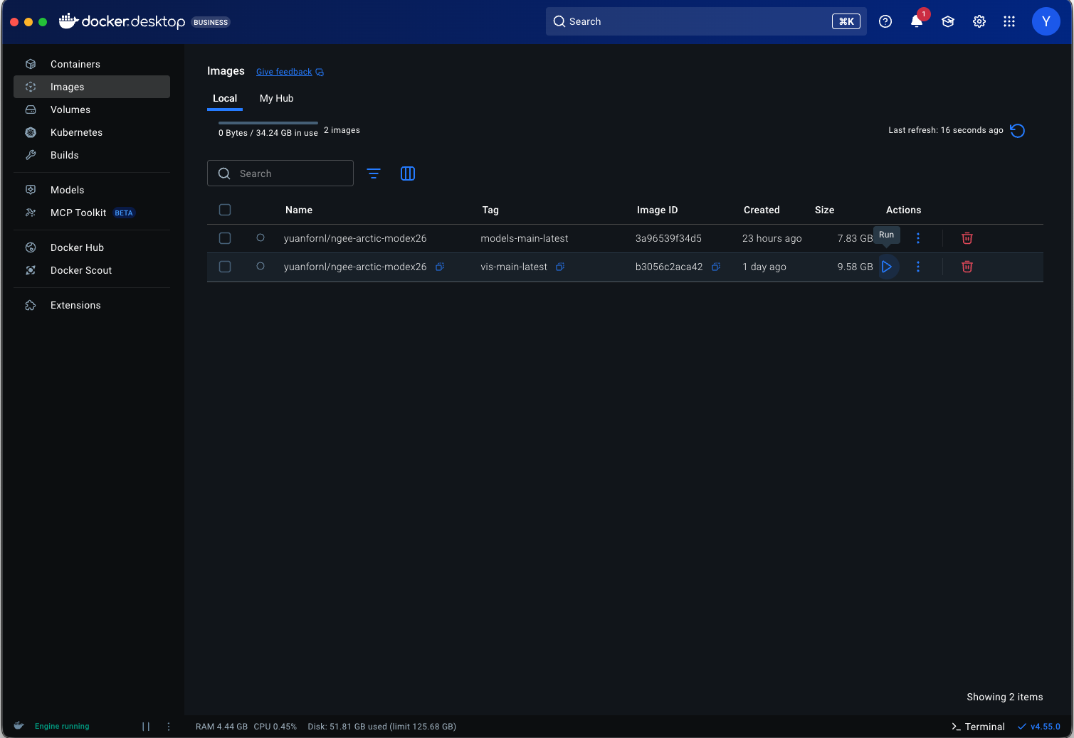
2. Click the Triangle run button next to the image ‘yuanfornl/ngee-arctic-modex26:vis-main-latest’ to start

   

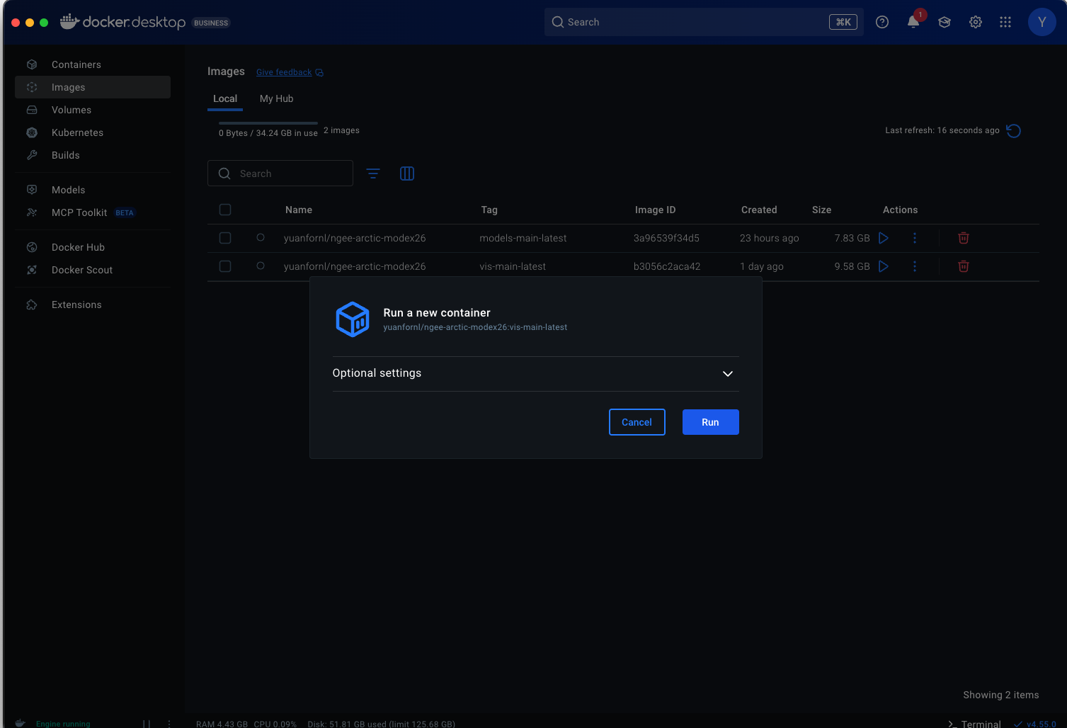
3. It will pop up a option/setting page, click and pull the drawdown button, and edit as following.

   

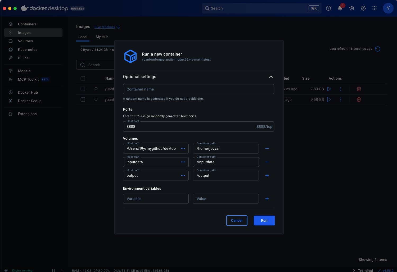
Note: The first row of volume hookup is for connecting Your local cloned repository ‘Field-to-Model’ directory (full path) to docker container’s directory of ‘/home/jovyan’.

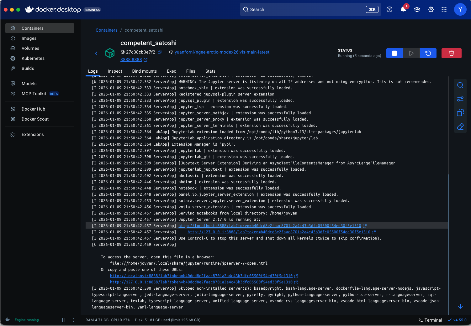
4. Click Run button and it will start Jupyter notebook. Notice the https links in the output and click on them to pop up a browser window.

   

5. In the pop-up browser window, it should show the landing page like following.

   

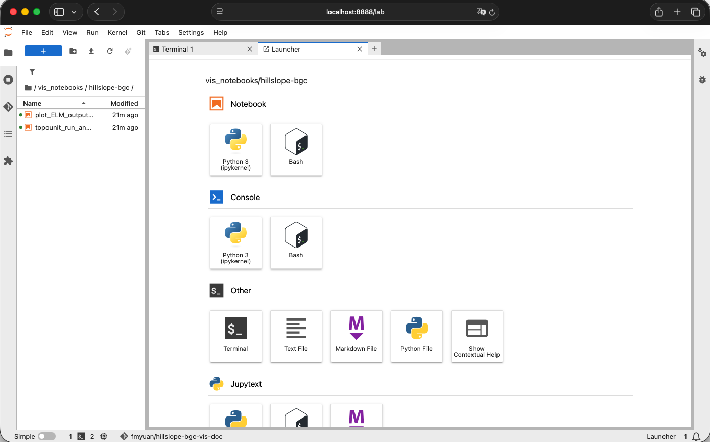
8.5.3. Visualizing results using jupyter notebook

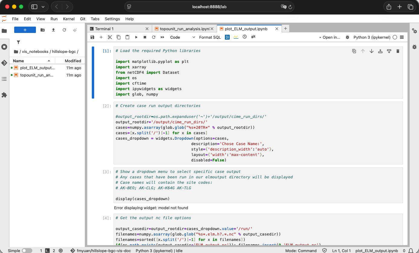
Click the left explorer window, and click-open the folder: /vis_notebooks/hillslope-bgc/

Click open file: plot_ELM_output.ipynb. We will run this script to open a ELM output file, and investigate a few variables.

8.5.4. Analyzing the impact of topounits and hillslope hydrology on hydrology (soil moisture) and biogeochemistry (GPP)

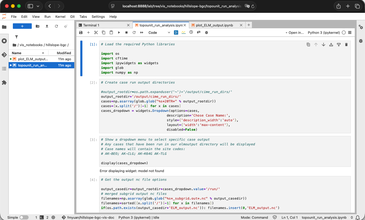
From the left explorer window, click-open file: topounit_run_analysis.ipynb. We will run this script to open merged_ncfile we created for 4 simulations in previous runs, and conduct some analysis.

We’re going to focus on two variables: top-10cm soil moisture and GPP.