4. Introduction to TEM and Warming Experiment Example
4.1. What are we trying to model?
NGEE Arctic has worked on numerous experiments and field equipment over the last decade+, one of which being the zero-power warming chambers (see Lewin et at. (2017) https://bg.copernicus.org/articles/14/4071/2017/bg-14-4071-2017.pdf) The chambers passively warm the mean daily temperature inside the chamber by 2.6◦C above ambient temperatures during the summer months. Modeling such field experiments allows us to evaluate how well the model is able to capture the ecosystem responses to warming, and thus how adequate the model is for predicting future ecosystem changes.
At Utqiagvik, the chambers were deployed over a single season in multiple locations from 2017-2021 from mid-June through to mid-September (Ely et al. 2024). In this example, we model the 2019 summer warming experiment and compare the modeled and measured soil temperatures at 10cm depth for the warmed and control site. The 2019 experiment focused on Eriophorum angustifolium, a common sedge species in Arctic tundra which in the model DVM-DOS-TEM is represented by the sedge plant functional type (PFT) and grows for example in the wet sedge tundra community type (CMT). We model the warming experiment at a single pixel representing the wet sedge tundra CMT at Utqiagvik and compare the soil temperature at 10cm depth between the control and warmed runs to the observed soil temperatures at the site (Ely et al. 2024).
Note
For the purposes of this workshop, DVM-DOS-TEM, dvmdostem, dvm-dos-tem and TEM synonymously refer to the “Dynamic Vegetation Model, Dynamic Organic Soil Terrestrial Ecosystem Model” which is the coupled vegetation and ecosystem model.
Lewin, K. F., McMahon, A. M., Ely, K. S., Serbin, S. P., & Rogers, A. (2017). A zero-power warming chamber for investigating plant responses to rising temperature. Biogeosciences, 14(18), 4071-4083.
Ely, Kim, Anderson, Jeremiah, Serbin, Shawn, & Rogers, Alistair (2024). Vegetation Warming Experiment: Thaw depth and dGPS locations, Utqiagvik, Alaska, 2019. https://doi.org/10.5440/1887568
4.2. Setup
4.2.1. Starting the container
Assuming you have completed all the step in the Getting Started instructions, run the following command to start a shell in the model container:
docker run -it --pull always --rm \
   -v $(pwd):/home/modex_user \
   -v inputdata:/mnt/inputdata \
   -v output:/mnt/output \
   yuanfornl/ngee-arctic-modex26:models-main-latest /bin/bash
Which should leave you at a shell prompt inside the container, like this:
modex_user@40bc0d780707:~$
This is your prompt and it will be shown in some of the following examples and
omitted in others. Note that your prompt shows your user name (modex_user),
and your current directory (the ~ symbol indicates your home directory). If
your prompt is shown in the examples, then you don’t need to type it - it’s just
there to show you where you are in the container.
Unless otherwise specified, all following commands should be run inside this
container. You can run the ls command to explore the contents of the
mounted volumes:
modex_user@1c2cffece04d:~$ ls /mnt/
inputdata  output
If you are able to see these two folders, then you have successfully mounted the volumes and are ready to proceed.
4.2.2. Inputs
Browse the data in the mounted /mnt/inputdata volume to see what is
available. You can think of the volume as hard drive that you have plugged in to
the container.
Check to see what datasets are available for TEM in the inputdata volume:
modex_user@40bc0d780707:~$ ls /mnt/inputdata/TEM/
cru-ts40_ar5_rcp85_ncar-ccsm4_toolik_field_station_10x10
modex26_1x1_AK-UTQ
These are the prepared input datasets for the TEM model. The following warming experiment (and any other experiments) can be applied to any of these datasets - just make sure to adjust the commands accordingly. For the purpose of this exercise we will focus on the Utqiagvik site (AK-UTQ).
About the input datasets...
TEM is in the process of re-vamping the input dataset production process. The
demo dataset that ships with the model is relatively old at this point (CRU
TS4.0; historic data only goes through 2015), and we are working on updating
it. This workshop will be the first test run of newly generated inputs that
are coming out of the new process. The new process is being developed as a
stand alone tool named temds which is being developed in this repo:
https://github.com/uaf-arctic-eco-modeling/Input_production
The (cru-ts40_ar5_rcp85_*_10x10/) datasets are the standard (old)
datasets that ship with the TEM model. Each dataset is a small 10x10 pixel
dataset that was made using the CRU TS4.0 climate data for historic climate
and the AR5 RCP8.5 projections from the NCAR CCSM4 model or MRI-CGCM3 for
future climate. These data were prepared originally for the IEM project but
have not been updated to more recent versions of CRU, so the historic data
ends in 2015.
The MODEX26 datasets (modex26_1x1_*) are single pixel datasets
prepared for the NGEE Arctic Modex workshop. These data were prepared from
recent CRU-JRA data, and downscaled with the delta method using WorldClim for
baseline and corrections. The projected (CMIP) data have not been processed,
though you will find placeholder files in the dataset folder. The historic
data goes from 1901-2023.
If you want to run some of the other datasets, you will probably want to read this info on run stages:
More info on TEM run stages...
TEM typically runs in multiple stages to cover the full historical and future periods. The typical stages are:
Equilibrium (EQ): Run model to reach a steady state using pre-industrial climate data.
Spinup (SP): Further spin-up using historical climate data.
Transient (TR): Run model with historical climate data from 1901 to present.
Scenario (SC): Run model with future climate projections from present to 2100.
By gluing the transient and scenario datasets together, we can simplify the run process into a single stage covering 1901-2100.
And this section on how to glue together transient and scenario datasets.
Advanced - gluing transient and scenario stages...
If you are using the cru-ts40_ar5_rcp85_*_10x10/ datasets you will find
that they have both historic and projected climate data files (though the
“projected data” covers the 2015-present time range - these are old
projections).
If you would like to use these files for the warming experiment and see what a run that projects into the future looks like you will need an additional step to glue the historic and projected datasets together. See the instructions in the next section for how to do this.
To make the experiment and analysis easier, we will glue together the
historic and projected (scenario) climate data into a single continuous dataset.
This will allow us to run the model in a single stage from 1901-2100 rather than
having to do a transient run followed by a scenario run. Use the helper script
in the model_examples/TEM directory to do this:
./model_examples/TEM/glue_transient_scenario.py \
   /mnt/inputdata/TEM/cru-ts40_ar5_rcp85_ncar-ccsm4_toolik_field_station_10x10
Now if you look in the new directory, you should see a new file called
stock-historic-climate.nc which is the original file that came with the
dataset. The file historic-climate.nc is now the glued together version
that covers 1901-2100. The same applies to the CO2 files.
modex_user@b86337d9ef42:~$ ls -1 \
   /mnt/inputdata/TEM/cru-ts40_ar5_rcp85_ncar-ccsm4_toolik_field_station_10x10/
co2.nc
drainage.nc
fri-fire.nc
historic-climate.nc
historic-explicit-fire.nc
notes.txt
original-vegetation.nc
projected-climate.nc
projected-co2.nc
projected-explicit-fire.nc
run-mask.nc
soil-texture.nc
stock-co2.nc
stock-historic-climate.nc
topo.nc
vegetation.nc
Examining a NetCDF file.
You can use the ncdump utility to inspect the contents of the new
netCDF file. Pass the -h flag to see the header information. For example:
ncdump -h /mnt/inputdata/TEM/cru-ts40_ar5_rcp85_ncar-ccsm4_toolik_field_station_10x10/historic-climate.nc
This will show you the dimensions and variables in the file, including the time dimension which should now span from 1901 to 2100.
4.2.3. Setting up the run folders
We are going to need two folders for this experiment - one for the control run and one for the warming treatment run. Each run folder will contain the necessary configuration files and output locations for the model to run.
We will use the pyddt-swd utility to create these run folders. This tool
sets up a “standard” run folder structure for the model, including copying over
necessary input files from the input dataset (see the --copy-inputs flag
below). Omit this flag if you want to link to the input files instead of copying
them. The way the files are linked is by setting the paths in the config file to
point to the absolute path of the source inputs. If you specify the
--copy-inputs flag, the input files are physically copied into the run
folder. Copying is safer in case the input dataset gets modified later, but it
does take more disk space.
For this we will create a new folder in the /mnt/output/ directory and
switch into it:
mkdir -p /mnt/output/tem/tem_ee1_warming
cd /mnt/output/tem/tem_ee1_warming

pyddt-swd \
   --input-data-path /mnt/inputdata/TEM/modex26_1x1_AK-UTQ \
   --copy-inputs \
   control
Hint
If you get an FileExistsError when running the above commands, it means
that the run folders already exist. You can either delete them and re-run the
commands, or provide the --force flag to overwrite the existing folders.
You should now have two run folders set up for the control and treatment runs:
modex_user@b86337d9ef42:/mnt/output/tem/tem_ee1_warming$ ls -l
total 4
drwxr-xr-x 6 modex_user modex_user 4096 Dec 12 19:41 control
Note
The -l flag to the ls command shows more detailed information about
the files and folders, including permissions, ownership, size, and modification
time.
4.2.4. Do the control run
There are a few more setup steps that need to be done before starting the control run.
Change into the run folder, e.g.
cd /mnt/output/tem/tem_ee1_warming/control.Explore the contents of this folder. Note that you should have a run-mask, config folder, and an output folder already created by the
pyddt-swdcommand. Also in the config folder you should find a file calledoutput_spec.csvwhich is the output specification file that tells the model which variables to output.Set the run mask (if you have a single pixel dataset, you can skip this step).
Advanced - using the run mask for multi-pixel datasets
Some of the inputs are single pixel while others are multi-pixel datasets. If you have a multi-pixel dataset, you may want to adjust the run mask so that only a subset of pixels are active for the run. This is especially useful for workshop exercises where we want to keep the run time short and the output data size small.
The run mask file in an input data folder (
run-mask.nc) controls which pixels are active in the model run. A value of 1 indicates that the pixel is active, and a value of 0 indicates that the pixel is inactive.We will use the
pyddt-runmaskutility to adjust the run mask so that only the desired pixel is active for this run.For this example, we will enable only the pixel at (0,0) - the first pixel in the dataset.
pyddt-runmask --reset --yx 0 0 run-mask.nc
Note
See the
--helpmessage for more options on how to select pixels.Setup the output specification file. This is a
csvfile that tells the model which variables to output and at what resolution. You can edit it by hand but it’s easier to use thepyddt-outspecutility to add the variables you want. There are many variables to choose from - for this example, we will output GPP (Gross Primary Productivity), LAYERDZ (layer thickness), and TLAYER (temperature by layer). We will also enable the CMTNUM variable to help identify the community type in the generated outputs. This ispyddt-outspec config/output_spec.csv --on GPP m p pyddt-outspec config/output_spec.csv --on LAYERDZ m l pyddt-outspec config/output_spec.csv --on TLAYER m l pyddt-outspec config/output_spec.csv --on CMTNUM y # Print it out to confirm what vars we have at what resolution... # Hint: you need a wide terminal for this to look good! pyddt-outspec config/output_spec.csv -s Name Units Yearly Monthly Daily PFT Compartments Layers Data Type Description CMTNUM m y invalid invalid invalid invalid invalid int Community Type Number GPP g/m2/time y m invalid p invalid double GPP LAYERDZ m y m invalid invalid invalid l double Thickness of layer TLAYER degree_C y m invalid invalid invalid l double Temperature by layer
Optional - config file settings.
Advanced - adjusting config file settings
The config file is a
jsonfile that contains a bunch of settings for the run. You may want to look through the file to see what things are available for changing. You can edit the file directly with a text editor, or you can use a small script to do it programmatically or in an interactive Python session, as in the following example.cd /mnt/output/tem/tem_ee1_warming/control/ ipython Python 3.11.14 | packaged by conda-forge | (main, Oct 13 2025, 14:09:32) [GCC 14.3.0] Type 'copyright', 'credits' or 'license' for more information IPython 9.6.0 -- An enhanced Interactive Python. Type '?' for help. Tip: Put a ';' at the end of a line to suppress the printing of output. In [1]: import json In [2]: with open('config/config.js') as f: ...: jd = json.load(f) In [3]: jd['general']['output_global_attributes']['run_name'] = "Some kind of great name..." In [4]: with open('config/config.js', 'w') as f: ...: json.dump(jd, f, indent=4)
Now we can start the control run:
dvmdostem -f config/config.js -p 100 -e 1000 -s 250 -t 123 -n 0 --force-cmt 6 -l monitor
When you run this command you should eventually see the following output:
.. Setting up logging...
[monitor] [EQ] Equilibrium Initial Year Count: 1000
[monitor] [EQ] Running Equilibrium, 1000 years.
[monitor] [SP] Running Spinup, 250 years.
[monitor] [TR] Running Transient, 123 years
cell 0, 0 complete.
Total Seconds: 155
4.2.5. Do the warming/treatment run
There are a few more setup steps that need to be done before starting the control run.
Change directories up to the main experiment folder:
cd /mnt/output/tem/tem_ee1_warming
Make a new run folder for the warming treatment if you have not already done so. Here we name it with a descriptive name indicating the treatment:
pyddt-swd \
   --input-data-path /mnt/inputdata/TEM/modex26_1x1_AK-UTQ \
   --copy-inputs \
   warming_2.6C_JJAS_2019
Change into the run folder, e.g.
cd /mnt/output/tem/tem_ee1_warming/warming_2.6C_JJAS_2019.Modify the input dataset to create the warming treatment dataset.
We will use a helper script to modify the air temperature variable in the climate data file to add 2.6 degrees Celsius during the summer months (June, July, August, September) for the year 2019.
python /home/modex_user/model_examples/TEM/modify_air_temperature.py \
--input-file inputs/modex26_1x1_AK-UTQ/historic-climate.nc \
--months 6 7 8 9 \
--years 2019 \
--deviation 2.6
Details about the modification script
The modification script uses
xarrayunder the hood to manipulate the netCDF data. It creates a boolean mask for the time dimension based on the specified years and months, and then applies the temperature deviation only to those selected time points.The modification script can take additional arguments to modify multiple years and different months as needed. See the help message for details.
As you will see in the statements that are printed out from this script it will actually create an new file (
modified_historic-climate.nc) alongside the existing one (historic-climate.nc). Here we throw out the original file and rename the modified version to clean things up.mv inputs/modex26_1x1_AK-UTQ/modified_historic-climate.nc inputs/modex26_1x1_AK-UTQ/historic-climate.nc
Note
If for some reason you want to keep the original file, rather than removing it, you can simply update the path in the config file to point to the modified file instead.
Examining the modified data
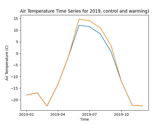
You can make a plot of the air temperature variable to confirm that the modification worked as expected. Use the
xarraylibrary in a Python session to load the modified dataset and plot the air temperature time series.Note
You can run this code in visualization container - it has IPython and all the visualization libraries installed.
import xarray as xr
import matplotlib.pyplot as plt

# Load the modified dataset
ds_control = xr.open_dataset(
   '/mnt/output/tem/tem_ee1_warming/control/inputs/modex26_1x1_AK-UTQ/historic-climate.nc'
)
ds_warming = xr.open_dataset(
   '/mnt/output/tem/tem_ee1_warming/warming_2.6C_JJAS_2019/inputs/modex26_1x1_AK-UTQ/historic-climate.nc'
)

# Select the air temperature variable (assuming it's called 'tair')
tair_control = ds_control['tair']
tair_warming = ds_warming['tair']

# Plot the time series for 2019
for ds, label in zip([tair_control, tair_warming], ['control', 'warming']):
   ds_2019 = ds.sel(time=slice('2019-01-01', '2019-12-31'))
   ds_2019[:,0,0].plot(label=label)

plt.title('Air Temperature Time Series for 2019, control and warming)')
plt.xlabel('Time')
plt.ylabel('Air Temperature (C)')
plt.savefig('air_temperature_2019.png')
This should produce a plot showing the air temperature time series for 2019, with the warming dataset showing a 2.6C increase during the summer months (June-September). It should look something like this:
Set the run mask - same as for the control run.
Setup the output specification file - same as for the control run, or simplify copy the file from the control run folder.
cp ../control/config/output_spec.csv config/output_spec.csv
Optional - config file settings, same as for the control run.
Start the warming run - same command as for the control run!
Hint
Make sure you are in the warming run folder before starting the run!
dvmdostem -f config/config.js -p 100 -e 1000 -s 250 -t 123 -n 0 -l monitor --force-cmt 6
4.3. Analysis
For the analysis portion of this experiment, we will use a Jupyter Notebook to visualize and compare the outputs from the control and warming runs. This allows us to interactively explore the data and create plots to see how the warming treatment affected the soil temperatures.
To start this notebook, use another terminal to launch a Jupyter Notebook server in a new container:
docker run -it --pull always --rm \
   -p 8888:8888 \
   -v $(pwd):/home/jovyan \
   -v inputdata:/mnt/inputdata \
   -v output:/mnt/output \
   yuanfornl/ngee-arctic-modex26:vis-main-latest
You should see output like this:
[I 2025-12-12 21:31:22.299 ServerApp] jupyter_lsp | extension was successfully linked.
[I 2025-12-12 21:31:22.305 ServerApp] jupyter_server_terminals | extension was successfully linked.
[I 2025-12-12 21:31:22.311 ServerApp] jupyterlab | extension was successfully linked.
[I 2025-12-12 21:31:22.317 ServerApp] notebook | extension was successfully linked.
...
    To access the server, open this file in a browser:
     file:///home/jovyan/.local/share/jupyter/runtime/jpserver-360-open.html
 Or copy and paste one of these URLs:
     http://2aecc7b15434:8888/tree?token=e66b3be47f2b3d7721adeb88992b8b1818901c5d76281678
     http://127.0.0.1:8888/tree?token=e66b3be47f2b3d7721adeb88992b8b1818901c5d76281678
Once the server is running, you should see a URL printed out in the terminal
that you can open in your web browser on your host computer to access the
Jupyter interface. Navigate to the vis_notebooks/TEM/ directory and
open the temperature_plotting.ipynb notebook.
Note
TODO make sure all this is in the notebook…
What kinds of plots and analyses do we want to provide? What variables are we most interested in? How do we want to visualize the differences between the control and warming runs?
Some ideas:
Time series plots of key variables (e.g. GPP, NEE, soil carbon) for control vs warming
Seasonal cycle plots
Difference maps if multi-pixel
Statistical summaries (means, variances, trends)
Comparison to observational data if available